Frank Pattyn
Home | C.V. | Research | Publications | Cours | Leisure | Contact
|
Frank PattynHome | C.V. | Research | Publications | Cours | Leisure | Contact |
GRANTISM is an educational numerical model of the Greenland & Antarctica ice sheet, programmed in Microsoft Excel and is approximately 100 Kb in size. The model allows the user to simulate both ice sheets along a central flow line, as a function of the background temperature, and hence under a number of climatic scenario's. The model is completely thermomechanically coupled, and includes isostatic adjustment. Starting from the present observed bedrock topography and specific accumulation pattern reigning over both continents, a mathematical ice sheet will build up until a steady-state (equilibrium) condition is reached. Two parameters can be changed by the user to control the model (see below).
Recent climate studies show that global temperature rises and that this trend will continue in the following years to come. A climate warming could lead to a potential melting of ice masses on earth, such as mountain glaciers and ice sheets. Generally, ice is a good indicator for changes in the climate. Especially glaciers seem to react fast to changes in climate - they retreat with rising temperatures - which is relatively easy to monitor. In the European Alps, glaciers seem to have retreated more than one kilometer since the end of the nineteenth Century.
The response of the Antarctic ice sheet to changes in background temperature is likely to be different for the Greenland ice sheet. Because of the extremely cold surface temperatures across Antarctica, the ice sheet is considered to remain relatively stable for 100-year time scales under warming scenarios of up to 20ºC. This follows because the increased moisture content in warmer air masses leads to increased precipitation rates. The situation in Greenland is quite different. While inland surface temperatures are well below freezing, surface melting in the ablation zone presently accounts for roughly half of the mass loss from the Greenland ice sheet. The general consensus suggests that modest-to-moderate warming over the next millennium will lead to a gradual, dynamic interplay between marginal mass loss in the ablation zone and increased mass gain in the accumulation zone resulting in a slow, monotonic ice-sheet retreat.
To investigate the reaction of large ice sheets on changes in climate, we use mathematical models to simulate these changes in ice volume. A mathematical model is based on the physical characteristics of the ice and the deformation of the ice, which are expressed in mathematical formulas and using mathematical principles are translated to computer code.
Ice might be crystalline material, when subjected to prolonged stress it will deform, similar to any metal when brought close to its melting point. These stresses can develop due to an unequal distribution of weight, such as topography. A stake placed on the surface of a glacier will, due to deformation of the underlying ice column, move in the direction of the maximum surface slope. The relation between the deformational velocity (strain rate) of the ice and the exerted stress is called the flow law for ice and determined by a large number of experiments, in the laboratory as well as in the field:
Strain rate e = A(T) s3, where s = r g H sin a.
A(T) is a flow-law parameter which is dependent on the temperature of the ice. Cold ice (-50°C) will deform less than so-called warm ice (ice where its temperature is close to the melting point), which will have a higher viscosity. The stresses within the ice mass (s) are a function of the weight of the ice column (r g H, where r is the ice density, g the gravitational acceleration and H the ice thickness), and the surface slope (sin a). If ice would not deform, the Antarctic ice sheet would continually grow, given its positive surface mass balance due to snow accumulation. Due to motion and deformation, ice from the interior of the ice sheet is transported towards the coast, where it ends in the sea as an ice shelf, from which icebergs break off. The mean yearly snow accumulation thus forms a boundary condition in the model and ascertains a continuous input of ice to the system. The ice sheet reaches a steady-state condition when the input of snow/ice (accumulation) equals the total amount of ice loss at the edge of the ice sheet, due to calving of icebergs and melting (ablation). Any imbalance will make the ice sheet grow or shrink.
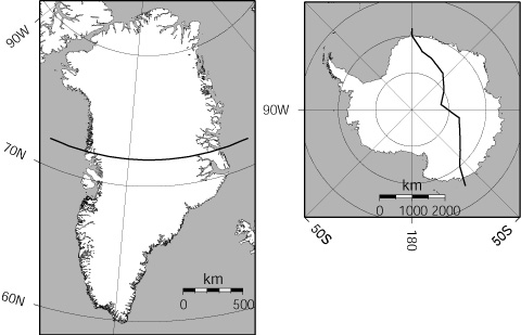
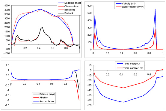
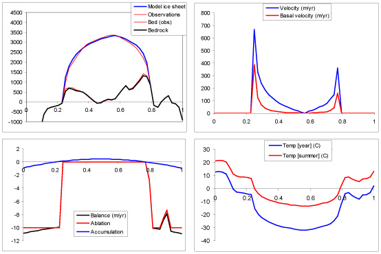
The GRANTISM model enables you to carry out climate experiments with the Greenland and Antarctic ice sheet. The model is completely based on the physical principles described above. More detailed information on the model description and its numerics are found here. Boundary conditions to the model are snow accumulation at the surface and yearly mean surface temperature. The model is a so-called flowline model, i.e. the ice sheet is simulated along a flowline running through the central part of the present ice sheet (Figure 1). Two parameters may be changed by the user. These are:
RUN = 0, 1 or 2. This parameter permits the model to run. The model starts initially from the present basal topography of the ice sheet, without ice and isostatically adjusted for the lack of ice (RUN = 0). You can also start from the present ice-sheet conditions by setting RUN = 2. If subsequently RUN is set to 1 (type 1 in the appropriate cell, followed by <ENTER> to validate your choice), every year another layer of ice (snow) will be added to the model. The thickness of this layer is determined by the yearly amount of accumulation. Generally, accumulation is higher at the coast than in the center of the ice sheet. The model time step is 200 years for the Antarctic ice sheet, and when you let the model run, 20 iterations are carried out at once (= 4000 years). You have to press F9 a number of times (each time another 20 iterations are carried out) before the ice sheet reaches a steady-state condition. For an Apple Mac computer press the command button together with the = button, i.e. <COMMAND>+<=>. When the ice sheet is in steady state the volume does not change anymore and should mark 100% for the standard experiment.
TFOR. This parameter controls the changes in global mean (background) air temperature. For simulating the present environmental conditions, TFOR = 0. Before running the model with a particular value, one starts best with RUN set to 0 or 2, then assigning a value for TFOR, and subsequently setting RUN equal to 1. Use the F9 button to bring the model ice sheet to a new equilibrium.
Optional parameters are listed in the spreadsheet below the control parameters. They are BASALSL, TKOPP, DATASET, BEDADJ, and SEALEV. BASALSL controls basal sliding in the model. Set to 0, the ice sheet remains frozen to the bed (default = 1). TKOPP introduces the ice-temperature coupling, otherwise an isothermal ice sheet is considered (default = 1). DATASET selects the model domain: 1 stands for the Antarctic ice sheet, 2 for Greenland and 0 for a initial flat bedrock (ideal ice sheet). BEDADJ controls isostatic bed adjustment (default = 1, activated). Finally, SEALEV introduces the sea-level lowering for colder background temperatures associated with the formation of Northern Hemisphere ice sheets (default = 1).
Circular reference error: in the TOOLS menu, go to OPTIONS. Choose CALCULATION and thick the box in front of ITERATION.
Changing the iteration scheme: in the TOOLS menu, go to OPTIONS. Choose CALCULATION and set maximum iterations.
Changing values in the spreadsheet: go to the sheet of interest (Model or Calculations) and select all cells (CTRL+A). In the DATA menu, choose VALIDATION. Check CLEAR ALL. Now you can edit the spreadsheet.
What kind of experiments should you carry out? Well, let the model run with different values for TFOR, e.g. -10, -5, 0, 5, 10, 15 and 20°C. Write down your findings, i.e. what is the ice volume for each of these experiments (in percentage of the present steady-state value); what is the surface temperature in the center of the ice sheet and at the edge (coast); what is the accumulation / ablation at these areas, ... Afterwards you can analyse you findings and try to explain some of them. Here follow some hints: